Green, Gauss, Stokes: the classical theorems of integral calculus (part II)
This time we'll go over the Green and Stokes theorems in a similar way. In the interpretation of a vector field $V$ as the velocity field of some fluid, while the divergence measures the rate at which the fluid diverges (i.e. flows away) from a point $p$, the curl measures the rate at which the fluid curls (i.e. circulates) around $p$. This leads to a subtler notion because a fluid could circulate around any axis through $p$ (or, in dimensions greater than $3$, circulate within any plane through $p$), so we'll begin by looking at the plane only.
So let $V$ be a vector field on the plane $\mathbb{R}^2$, and $p$ a point in $\mathbb{R}^2$. How do we quantify this curling around $p$? We take a disk $D(p; \epsilon)$, with boundary circle oriented counter-clockwise, and look at \[ \int_{\partial D(p; \epsilon)} V \cdot ds \] The integrand $V \cdot ds$ gives us the tangential component of velocity, which is what makes the fluid go around the circle -- so integrating it gives the total circulation (this can be more precisely interpreted as the total angular momentum of the circle). To define the curl we do as we've been doing and set \[ (\text{curl}\ V)(p) = \lim_{\epsilon \to 0} \frac{1}{\text{vol}(D(p; \epsilon))} \int_{\partial D(p; \epsilon)} V \cdot ds \] Exercise: Show that, for $V = (V^1(x,y), V^2(x,y))$, \[ \text{curl}\ V = \frac{\partial V^2}{\partial x} - \frac{\partial V^1}{\partial y} \] with the same strategy as before, i.e. taking $p = (0, 0)$ and using the Taylor approximation \[ V(x, y) \approx V(0, 0) + \left( x \frac{\partial V^1}{\partial x}(0, 0) + y \frac{\partial V^1}{\partial y}(0, 0), x \frac{\partial V^2}{\partial x}(0, 0) + y \frac{\partial V^2}{\partial y}(0,0) \right) \]
Then we get Green's theorem in a very similar way:
Theorem (Green): Let $U \subset \mathbb{R}^2$ be a region with piecewise differentiable boundary, oriented counter-clockwise, and $V$ a $C^2$ vector field. Then \[ \int_U \text{curl}\ V\ dx dy = \int_{\partial U} V \cdot ds \] Proof (heuristic): The limit definition of curl also works for any piecewise differentiable shape shrinking to our point. So we subdivide the region $U$ into very small (counter-clockwise oriented) triangles again: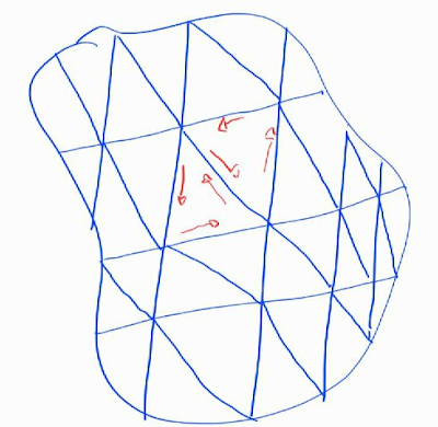 The proof is then exactly the same as before. Over each triangle $\Delta$ we use the approximation
\[ \text{curl}\ V \approx \frac{1}{\text{vol}(\Delta)} \int_{\partial \Delta} V \cdot ds \]
Therefore
\[ \int_{U} \text{curl}\ V\ dx dy = \sum_{\Delta} \int_{\Delta} \text{curl}\ V\ dx dy \approx \sum_{\Delta} \int_{\partial \Delta} V \cdot ds\]
The integral of $V \cdot ds$ over each internal side is performed twice with opposite orientations, and so cancels out, and we're left with only the boundary terms. Taking the limit as the subdivision gets finer we obtain
\[ \int_{U} \text{curl}\ V\ dx dy = \int_{\partial U} V \cdot ds\]
as desired. $\square$
The proof is then exactly the same as before. Over each triangle $\Delta$ we use the approximation
\[ \text{curl}\ V \approx \frac{1}{\text{vol}(\Delta)} \int_{\partial \Delta} V \cdot ds \]
Therefore
\[ \int_{U} \text{curl}\ V\ dx dy = \sum_{\Delta} \int_{\Delta} \text{curl}\ V\ dx dy \approx \sum_{\Delta} \int_{\partial \Delta} V \cdot ds\]
The integral of $V \cdot ds$ over each internal side is performed twice with opposite orientations, and so cancels out, and we're left with only the boundary terms. Taking the limit as the subdivision gets finer we obtain
\[ \int_{U} \text{curl}\ V\ dx dy = \int_{\partial U} V \cdot ds\]
as desired. $\square$
As mentioned previously, the generalization of Green's theorem to three dimensions (known as Stokes's theorem) has the extra subtlety that the curling can be about any axis. This is really better understood in the language of differential forms (since it's more proper to think of rotations as happening in a plane, rather than being about an axis), but for the sake of completeness I'll show how to do this in the elementary calculus language we've been using.
For a vector field $V$ on $\mathbb{R}^3$, the idea is to think of $\text{curl}\ V$ as a vector field itself, whose $x$ component at a point $p$ is the curl of $V$ about the $\hat{x}$ axis through $p$, and similarly for the other components. To get the formula right, we have to worry a little bit about orientations. In the two-dimensional case, in the definition of curl we integrated $V \cdot ds$ along a circle oriented counter-clockwise, and after taking the limit we obtained
\[\text{curl}\ V = \frac{\partial V^2}{\partial x} - \frac{\partial V^1}{\partial y}\]
In the three-dimensional case, this will be the curl about the $\hat{z}$ axis, i.e. the $z$ component of $\text{curl}\ V$. The sign is correct because orienting the $xy$ plane with the $\hat{z}$ normal does indeed lead to the notion of counter-clockwise as in the picture[1]. Equivalently, we might say this as $\hat{x} \times \hat{y} = \hat{z}$. Therefore, for $V = (V^1(x,y,z),V^2(x,y,z),V^3(x,y,z))$ we have
\[(\text{curl}\ V)_z = \frac{\partial V^2}{\partial x} - \frac{\partial V^1}{\partial y}\]
Similarly, since $\hat{y} \times \hat{z} = \hat{x}$, it follows the $x$ component of $\text{curl}\ V$ works out mutatis mutandis:
\[(\text{curl}\ V)_x = \frac{\partial V^3}{\partial y} - \frac{\partial V^2}{\partial z}\]
However, $\hat{x} \times \hat{z} = -\hat{y}$. So if we want to measure curling about the $\hat{y}$ axis, we need to think of the $xz$ plane as having $\hat{z}$ as its first direction, followed by $\hat{x}$. Therefore the sign gets switched:
\[(\text{curl}\ V)_y = \frac{\partial V^1}{\partial z} - \frac{\partial V^3}{\partial x}\]
(The rule we're following is: derivative of the second component with respect to the first direction, minus the derivative of the first component with respect to the second direction) So we get the usual formula
\[ \text{curl}\ V = \left( \frac{\partial V^3}{\partial y} - \frac{\partial V^2}{\partial z}, \frac{\partial V^1}{\partial z} - \frac{\partial V^3}{\partial x}, \frac{\partial V^2}{\partial x} - \frac{\partial V^1}{\partial y} \right) \]
which can be helpfully remembered as $\nabla \times V$.
In the two-dimensional case, in the definition of curl we integrated $V \cdot ds$ along a circle oriented counter-clockwise, and after taking the limit we obtained
\[\text{curl}\ V = \frac{\partial V^2}{\partial x} - \frac{\partial V^1}{\partial y}\]
In the three-dimensional case, this will be the curl about the $\hat{z}$ axis, i.e. the $z$ component of $\text{curl}\ V$. The sign is correct because orienting the $xy$ plane with the $\hat{z}$ normal does indeed lead to the notion of counter-clockwise as in the picture[1]. Equivalently, we might say this as $\hat{x} \times \hat{y} = \hat{z}$. Therefore, for $V = (V^1(x,y,z),V^2(x,y,z),V^3(x,y,z))$ we have
\[(\text{curl}\ V)_z = \frac{\partial V^2}{\partial x} - \frac{\partial V^1}{\partial y}\]
Similarly, since $\hat{y} \times \hat{z} = \hat{x}$, it follows the $x$ component of $\text{curl}\ V$ works out mutatis mutandis:
\[(\text{curl}\ V)_x = \frac{\partial V^3}{\partial y} - \frac{\partial V^2}{\partial z}\]
However, $\hat{x} \times \hat{z} = -\hat{y}$. So if we want to measure curling about the $\hat{y}$ axis, we need to think of the $xz$ plane as having $\hat{z}$ as its first direction, followed by $\hat{x}$. Therefore the sign gets switched:
\[(\text{curl}\ V)_y = \frac{\partial V^1}{\partial z} - \frac{\partial V^3}{\partial x}\]
(The rule we're following is: derivative of the second component with respect to the first direction, minus the derivative of the first component with respect to the second direction) So we get the usual formula
\[ \text{curl}\ V = \left( \frac{\partial V^3}{\partial y} - \frac{\partial V^2}{\partial z}, \frac{\partial V^1}{\partial z} - \frac{\partial V^3}{\partial x}, \frac{\partial V^2}{\partial x} - \frac{\partial V^1}{\partial y} \right) \]
which can be helpfully remembered as $\nabla \times V$.
In summary, $\hat{x} \cdot (\text{curl}\ V)$ gives you the curling about $\hat{x}$, and so on for $\hat{y}$ and $\hat{z}$. It's reasonable, then, to guess that this works for any axis: $\hat{n} \cdot (\text{curl}\ V)$ is the curl of $V$ measured in the plane perpendicular to $\hat{n}$. This fact becomes clearer in the language of differential forms (and I will suggest formal references in future posts), so I won't try to justify it.
Theorem (Stokes): If $\Sigma \subset \mathbb{R}^3$ is a surface with piecewise differentiable boundary, and $V$ a $C^2$ vector field, then \[ \int_{\Sigma} (\text{curl}\ V) \cdot \hat{n}\ d\Sigma = \int_{\partial \Sigma} V \cdot ds \] Proof (heuristic): It's the same basic idea: subdivide $\Sigma$ into many extremely small (curved) triangles. For a fine enough subdivision, each triangle $\Delta$ can considered to be basically flat (i.e. lie on the plane perpendicular to $\hat{n}$), and so we'll have the approximation \[ \frac{1}{\text{vol} (\Delta)} \int_{\partial \Delta} V \cdot ds \approx (\text{curl}\ V) \cdot \hat{n} \] Summing over all triangles, the same cancellation effect occurs and we're left with only the boundary terms, establishing \[ \int_{\Sigma} (\text{curl}\ V) \cdot \hat{n}\ d\Sigma = \int_{\partial \Sigma} V \cdot ds \] as desired. $\square$
Next time we'll start porting this over to the language of differential forms and integration on manifolds.
Green's theorem
So let $V$ be a vector field on the plane $\mathbb{R}^2$, and $p$ a point in $\mathbb{R}^2$. How do we quantify this curling around $p$? We take a disk $D(p; \epsilon)$, with boundary circle oriented counter-clockwise, and look at \[ \int_{\partial D(p; \epsilon)} V \cdot ds \] The integrand $V \cdot ds$ gives us the tangential component of velocity, which is what makes the fluid go around the circle -- so integrating it gives the total circulation (this can be more precisely interpreted as the total angular momentum of the circle). To define the curl we do as we've been doing and set \[ (\text{curl}\ V)(p) = \lim_{\epsilon \to 0} \frac{1}{\text{vol}(D(p; \epsilon))} \int_{\partial D(p; \epsilon)} V \cdot ds \] Exercise: Show that, for $V = (V^1(x,y), V^2(x,y))$, \[ \text{curl}\ V = \frac{\partial V^2}{\partial x} - \frac{\partial V^1}{\partial y} \] with the same strategy as before, i.e. taking $p = (0, 0)$ and using the Taylor approximation \[ V(x, y) \approx V(0, 0) + \left( x \frac{\partial V^1}{\partial x}(0, 0) + y \frac{\partial V^1}{\partial y}(0, 0), x \frac{\partial V^2}{\partial x}(0, 0) + y \frac{\partial V^2}{\partial y}(0,0) \right) \]
Then we get Green's theorem in a very similar way:
Theorem (Green): Let $U \subset \mathbb{R}^2$ be a region with piecewise differentiable boundary, oriented counter-clockwise, and $V$ a $C^2$ vector field. Then \[ \int_U \text{curl}\ V\ dx dy = \int_{\partial U} V \cdot ds \] Proof (heuristic): The limit definition of curl also works for any piecewise differentiable shape shrinking to our point. So we subdivide the region $U$ into very small (counter-clockwise oriented) triangles again:

Stokes's theorem
As mentioned previously, the generalization of Green's theorem to three dimensions (known as Stokes's theorem) has the extra subtlety that the curling can be about any axis. This is really better understood in the language of differential forms (since it's more proper to think of rotations as happening in a plane, rather than being about an axis), but for the sake of completeness I'll show how to do this in the elementary calculus language we've been using.
For a vector field $V$ on $\mathbb{R}^3$, the idea is to think of $\text{curl}\ V$ as a vector field itself, whose $x$ component at a point $p$ is the curl of $V$ about the $\hat{x}$ axis through $p$, and similarly for the other components. To get the formula right, we have to worry a little bit about orientations.

In summary, $\hat{x} \cdot (\text{curl}\ V)$ gives you the curling about $\hat{x}$, and so on for $\hat{y}$ and $\hat{z}$. It's reasonable, then, to guess that this works for any axis: $\hat{n} \cdot (\text{curl}\ V)$ is the curl of $V$ measured in the plane perpendicular to $\hat{n}$. This fact becomes clearer in the language of differential forms (and I will suggest formal references in future posts), so I won't try to justify it.
Theorem (Stokes): If $\Sigma \subset \mathbb{R}^3$ is a surface with piecewise differentiable boundary, and $V$ a $C^2$ vector field, then \[ \int_{\Sigma} (\text{curl}\ V) \cdot \hat{n}\ d\Sigma = \int_{\partial \Sigma} V \cdot ds \] Proof (heuristic): It's the same basic idea: subdivide $\Sigma$ into many extremely small (curved) triangles. For a fine enough subdivision, each triangle $\Delta$ can considered to be basically flat (i.e. lie on the plane perpendicular to $\hat{n}$), and so we'll have the approximation \[ \frac{1}{\text{vol} (\Delta)} \int_{\partial \Delta} V \cdot ds \approx (\text{curl}\ V) \cdot \hat{n} \] Summing over all triangles, the same cancellation effect occurs and we're left with only the boundary terms, establishing \[ \int_{\Sigma} (\text{curl}\ V) \cdot \hat{n}\ d\Sigma = \int_{\partial \Sigma} V \cdot ds \] as desired. $\square$
Next time we'll start porting this over to the language of differential forms and integration on manifolds.
Notes
[1] To see this, imagine the $xy$ plane with the $\hat{z}$ normal pointing towards you -- your perspective defines counter-clockwise in said plane. ↩


Comments
Post a Comment